Information Field Theory I

(This post can also be seen here).

The thing that drew me back into theoretical physics was the need to learn Information Field Theory (IFT) for some of my current research on detecting the (very faint) radio emission associated with the large-scale structure of the universe (an older paper on the subject is here). IFT is basically Bayesian statistics applied to fields, but in certain cases the a posteriori probability can be computed through perturbation theory. Feynman diagrams can be used to compute the expansion (below are examples of a few terms), so I was forced to go back to my QFT book to remember the basics of perturbation theory….which led me back to QFT in general…. so here I am.

So what is IFT and why does it look a lot like QFT? I haven’t yet talked about QFT, but I can begin to explain IFT, at least the basics.

Consider a signal $s=s(x)$ , which is a function of position (a classical field), and we wish to make some inference about this field based on observational data $d$ . A common inference would be to make an image (map) from incomplete data. We model our measurement process as $d=Rs+n$ , were R is an operator describing the coupling between the data and signal, and n is random noise. Typically $s(x)$ is continuous and $d$ is discrete, so R will be some sort of selection function. It can also include more complicated transformations (e.g., Fourier transformations in the case of radio astronomy). In most cases, $n$ is gaussian, but it need not be.

We don’t know what the actual signal is, so $s$ is really just our model of what we think the signal is. In this case we’d like to compute the a posteriori probability that our model $s$ is the correct one given the data, denoted by $P(s|d)$ . Bayes’ theorem tells us that

$P(s|d)=\frac{P(d|s) P(s)}{P(d)}$

where $P(d|s)$ is the probability of getting $d$ given $s$ , called the likelihood, $P(s)$ is the prior probability of model $s$ , and $P(d)$ is the evidence, which is the normalization factor given by

$P(d) = \int \mathcal{D}s P(d|s) P(s)$ .

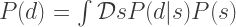
The integral is a functional integral of the likelihood over all possible configurations of $s$ , weighted by the prior probability of that configuration $P(s)$ . The likelihood contains information about the measurement process, and is typically a function the model signal’s parameters. There’s a lot out there on Bayes’ theorem so I won’t talk about it here, but is can be derived from basic facts about probabilities and Aristotelian logic.

The step taken in Ensslin et al. (2009) is to rewrite Bayes’ theorem in the form

$P(s|d) = \frac{e^{-H}}{Z}$

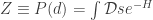where $H[s] \equiv -ln(P(d|s) P(s))$ is the Hamiltonian, and $Z \equiv P(d)=\int \mathcal{D}s e^{-H}$ . Things are starting to look suspiciously like statistical mechanics, where $Z$ is essentially the partition function; there are more links to stat. mech. that I can get into later. Let’s first consider an example.

Imagine that the signal we are trying to observe (make an image of) is a Gaussian random field (e.g., the cosmic microwave background fluctuations) denoted by $\mathcal{G}(s, S)$ . Let’s assume that the value of $s(x)$ at $x$ is not known, but we do know the signal covariance $S=<s s^{\dagger}>$ , i.e., the variance $\sigma^2$ of the Gaussian field. We can also assume that our observational noise is Gaussian $\mathcal{G}(n, N)$ (it often is), with an unknown value $n$ at any point, but with a known covariance $N = <n n^{\dagger}>$ . 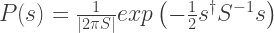In this case, the likelihood can be written as $P(d|s)=\mathcal{G}(d-Rs,N)$ and the prior probability is given by $P(s)=\mathcal{G}(s, S)$ ….. take a minute to convince yourself of this. In the case of the likelihood, if you assume $s$ is true, then the probability that you measure $d$ is going to depend on how far away $d$ is from $s$ , and will be a Gaussian. Explicitly, these are given by

$P(d|s)=\frac{1}{\vert 2\pi N \vert}exp\left( -\frac{1}{2}(d-Rs)^{\dagger}N^{-1}(d-Rs)\right)$

$P(s)=\frac{1}{\vert 2\pi S \vert}exp\left( -\frac{1}{2}s^{\dagger}S^{-1}s\right)$ .

This is all in matrix notation, where $\vert S \vert$ is the determinant of $S$ . As an exercise one can compute the Hamiltonian

$H[s]=-ln(P(d|s)P(s))=\frac{1}{2}s^{\dagger}D^{-1}s - j^{\dagger}s + H_{0}$ ,

where

$D= [S^{-1} + R^{\dagger}N^{-1}R]^{-1}$

is called the propagator of the free theory, and the information source $j$ is given by

$j = R^{\dagger}N^{-1}d$ .

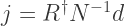The constant $H_{0}$ is the collection of all the terms independent of $s$ , is is given by

$H_{0}=\frac{1}{2} d^{\dagger}N^{-1}d + \frac{1}{2} ln( \vert 2 \pi S \vert \vert 2 \pi N \vert )$ .

To compute $P(s|d)$ , one just needs to plug in this Hamiltonian into Bayes’ theorem and compute the partition function integral. To obtain what we originally wanted, which was a map $m(x)$ of the signal $s(x)$ , we simply need to compute the expectation value of $s$ with respect to $P(s|d)$ , or

$m = <s>_{(s|d)} = \int \mathcal{D}s P(s|d) s$ .

This integral can be calculated in a number of ways. One way in particular is particularly useful for the perturbative extension of the theory, but for now one can compute directly that $m=Dj$ . In the continuous limit this reads

$m(x) = \int dy D(x,y)j(y)$ , and is represented by the diagram x y, where the external coordinate with no vertex is $x$ , the vertex coordinate is $y$ , and the line connecting them represents the propagator $D(x,y)$ . The vertex represents the information source $j(y)$ , and we should sum/integrate over the vertex (called internal later) coordinate. The intuitive understanding here is that $j$ contains all the data (projected onto the continuous space of the model, weighted by the noise via $j = R^{\dagger} N^{-1}d$ ), and $D(x,y)$ will “propagate” this information (it knows about the prior source covariance $S$ ) into unobserved parts of the map $m(x)$ .

All of this was already well understood in image reconstruction theory (in the form of a Wiener filter), but with the formalism of IFT, we can next look at what happens if we have higher order perturbations to the free theory Hamiltonian (and one often does!). Look for part II in the coming weeks.

2 Responses to Information Field Theory I

because0fbeauty says:

January 20, 2014 at 12:32 am

Shea,

I’d like to know more about the measure in those integrals, the $\mathcal{D}s$ . I’m woefully ignorant of measures in statistical mechanics but I suspect much of the rigorous treatment lies therein. On a barely related note, are you familiar with the “Riemann Gas” where by the particles are prime numbers and the partition function is the Riemann Zeta function?

- because0fbeauty says:
  
  January 20, 2014 at 12:34 am
  
  Oh, nevermind…looks like I have some reading to do, I missed the comment on functional integration.

	How to Carry a Bould… on Bikes and Boulders – Par…
	because0fbeauty on Context in mathematics
	sheabrowne on Reflections and Reports of Rep…
	sheabrowne on Reflections and Reports of Rep…
	because0fbeauty on Large numbers and abstraction…